pre-mba: facebook

Everyone admitted into the Oxford MBA program is immediately granted online access to the incoming-student intranet site. As time passes, more content is added. The intranet site is the primary way that administration communicates with us regarding scholarship winners, college availability, and student Q&A. It is also the best way to learn what Facebook page(s) have been created for each MBA class, so that students can begin to network, and get to know each other more informally.

Roughly two-thirds (158/240) of the incoming Oxford MBA class is on Facebook. Over the summer, many students have posted pre-MBA “meet-up” events in London, Mumbai, and New York. In fact, I helped organize the event in New York where I met two other Oxford-bound MBAs. Between the three of us, we worked at Barclays, Goldman Sachs, and Smith Barney. In addition to working in finance, two of us owned our businesses (one of which has secured a patent). From meeting other alumni I have learned that there will be two others joining us. That makes five of us from New York, which is about 10% of the US intake!

Make good use of the networking while you can. Many good schools offer solid MBA programs, and some students even skip the MBA altogether, and instead study for the Chartered Financial Analyst (CFA) designation. The difference lies in the people you meet, and the relationships you build, especially at a school like Oxford, which sets a very high threshold for admission.

In some of my earlier posts I mention that Oxford is divided into three terms (Michaelmas, Hilary, and Trinity). The first term begins on October 5th, and consists of six mandatory core courses: Finance I, Decision Science, Financial Reporting, Strategy I, Managerial Economics, and Marketing. MBA Students, however, must arrive on September 30^th for compulsory orientation. Unfortunately, college accommodations usually don’t start until October 1^st, which means that early-arrivers will have to pay a modest £18 per diem to move in earlier.

Come Hilary term, students get to choose three electives, and six more electives for Trinity term. To give you a flavor of the different electives available, the following classes were recently posted on the intranet site for Trinity term (I’ve highlighted the ones I’d like to take). If you feel like a kid in a candy store, then maybe you should apply to Oxford:

Business History, Business in China, Capital Raising, Cooperative Strategy, Corporate Valuation, CSR & Ethical Marketing, Customer Insight, Derivatives, Design Leadership, Environment Organizations & Sustainability, Financial Risk Management, Leading Strategic Change, Managing Complexity, Managing High-growth Companies, Managing the Project Portfolio, Marketing Innovation, Mergers Acquisitions & Restructuring, Negotiations, Private Equity, Real Estate, Retailing, Social Finance, Social Enterprise Design, Social Entrepreneurship and Innovation, Taxation Finance & Business Strategy, and Trading & Market Microstructure.

CFA study session #5: economics: macroeconomics (market structure)

Accepting that our resources are limited (aka factors of production: land, labor, capital, and entrepreneurship), the fundamental economic questions become: (1) what do we produce, (2) how do we produce it, and (3) how do we distribute it. Market theory, as originally developed by Adam Smith (student at Balliol College, Oxford) in his book the "Wealth of Nations (published 1776)," posits that the independent market forces of supply and demand provide the most efficient answers to these questions. That which should be produced is that for which people are willing to pay for. The method in which it should be produced is that method by which the lowest price to the consumer, and highest profit to the producer can be achieved. Further, such a product should be distributed to the highest bidder; those most willing to pay for it.

Adam Smith, however, presupposes that all such markets for goods and services exist in an ideal state, one in which there are many buyers and sellers, no barriers to entry, perfect information, and equal and undifferentiated products where the seller is a "price-taker." This may be true in some markets, such as when you buy a loaf of bread at the supermarket, but definitely not so when you are searching for competitors to upgrade your computer's Operating System. Macroeconomics investigates this range of different markets that actually exist:

Perfect Competition --> Monopolistic Competition

--> Oligopoly --> Monopoly

As we move from left to right the producer/seller gains the upper-hand. They often enjoy large market share, barriers to entry from competitors, and a differentiated product (quality, price, and marketing) that allows the firm to "price discriminate." Many countries, including the US, are unsure about the role of monopolies. Those that have enacted Anti-Trust legislation feel that monopolies stifle innovation and suffocate new companies from emerging. Economics worry that monopolies fail to satisfy consumer demand by producing at level below equilibrium so that they can maximize profits. Others argue that this is not the case. They think monopolies offer a superior product at a lower price than consumers would otherwise enjoy. some monopolies, such as Microsoft, are quite nimble, and their size affords them the ability to spend more money on R&D leading to greater discoveries. Before we can judge which structure is best for which market we need a way to categorize each industry.

The two methods used to determine which market structure a particular industry belongs to are the "Four-Firm Concentration Ratio" and the "Herfindahl-Hirschman Index (HHI)." Both are relatively easy to calculate. In the Four-Firm approach you simply calculate the percent of market share (by sales) controlled by the four largest firms in that industry. The range spans from 0% for perfect competition to 100% for a monopoly. Anything above 60% is considered an oligopoly.

For example, if we look up ExxonMobil (XOM) stock on Yahoo!Finance we can click on "Industry," and then "Industry Summary," and discover that ExxonMobil is in the "Major Integrated Oil & Gas" industry. We can also see that the top four companies by market capitalization are: ExxonMobil ($340B), PetroChina ($214B), Royal Dutch Shell ($165B), and British Petroleum ($160B). In total, the top four companies have a market capitalization of $879B. Meanwhile, the entire industry's market capitalization is $1,305B. Therefore, the Four-Firm ratio is 67.3% ($879B / $1,305B), and the "Major Integrated Oil & Gas" industry is considered an Oligopoly.

We use the Herfindahl-Hirschman Index when we require even greater specificity. The HHI adds the square of the percentage of market share of the top 50 firms in the industry (or all the firms if less than 50). To use a different example, if there are only four firms in an industry, and their market share (by sales) are: 50%, 25%, 15%, and 10% then we would use the formula:

HHI = 502 + 252 + 152 + 102 = 3,450 (Oligopoly)

Where the range is:

1 (perfect competition) --> 1,000 (monopolistic competition) --> 1,800 (oligopoly) --> 10,000 (monopoly)

***It should be disclosed that I used market capitalization to calculate both the Four-Firm ratio and Herfindahl-Hirschman Index as a proxy for market share by sales since I believe that there exists a high correlation between the two statistics, and because market capitalization data is more readily available.***

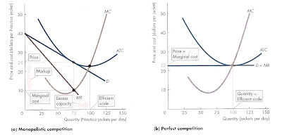
The following graphs are very useful in visually understanding the four types of market structures. The one thing they all have in common is that the equilibrium point is always found by first locating the intersection of Marginal Cost (MC) and Marginal Revenue (MR). In other words, firms always want to produce up until the point where manufacturing just one more unit no longer has any economic benefit, because the cost of producing that one additional unit outweighs the revenue generated. This will determine the equilibrium price and quantity.

Once we have found this point, we can find the equilibrium price by drawing an imaginary vertical line up to where it intersects with the Demand Curve (DC); follow the line downward to find the equilibrium quantity. Now that we know the price and quantity of that which is to be produced, we want to find out whether we are profitable. We determine profitability by once again following the imaginary vertical line that we have drawn to where it intersects with the Average Cost (AC) curve. The space between the DC and AC determines whether or not we have a profit or loss. We experience a profit if the AC lies below the DC. When AC lies above the DC we have an economic loss, and the firm should shutdown and cease operations.

Many of the examples we have used throughout this post have been oligopolies. The biggest fear when dealing with oligopolies is "price collusion," as most famously demonstrated by the oil cartel formed by OPEC during the 1970s. One way to combat oligopolies (or at least predict their behavior) is to apply game theory. When the strategies and payoffs for each player are known, and all players must follow the same rules, we can calculate the "Nash Equilibrium" for which outcome is most likely. The equilibrium depends on the nature of the game being played as there are several possible games, including the prisoners' dilemma and chicken. We expect more collusion to exist when a game is repeated, and "bad" behavior can be penalized, resulting in greater cooperation.

CFA study session #6: economics: monetary & fiscal policy

Earlier today US President Barack Obama nominated Ben Bernanke to a second term as US Federal Reserve Chairman after fierce controversy regarding his handling of the most severe economic recession in over thirty years. Obama had until January to make the decision. Previously, some speculated that Bernanke might be replaced by Larry Summers who had served in the Clinton administration, and later became President of Harvard University. So, to commemorate Bernanke's success I am posting a blog on monetary & fiscal policy.

After finishing the CFA Volume 2 (Economics) textbook, I am convinced that anyone having taken some introductory economic courses during college will do fine. Further, of the three study sessions found in Volume 2, I believe that macroeconomics will prove more difficult for most readers than the sections on microeconomics and government monetary & fiscal policy.

The most important take-aways on the readings regarding monetary & fiscal policy is that like many other central banks, the US Federal Reserve (Fed) focuses like a laser beam on one principle policy goal: to achieve economic growth with full employment, low inflation, and price stability. To guage the level of economic growth the Fed often looks at changes in the "gross domestic product (GDP)," which represents all the goods produced within the US in a given year. GDP is typically calculated through the "expenditure approach":

GDP = C + I + G + X
C = consumer spending
I = capital expenditures
G = government spending
X = net exports

Like a giant ship navigating through the ocean, the Fed uses monetary policy, accompanied by fiscal policy orchestrated by the US Treasury, to make constant minor adjustments to keep the economy on track. Unfortunately, incremental changes taken on a large ship often take a while before you can see a correction run its course and right the ship. Similarly, government policy often suffers from several time lags, including recognition (it takes time to realize something is wrong), law-making (it takes time to pass the necessary legislation), and impact (it takes time for the solution to work its way through the system). This brings us to the first, and most important, question of how we recognize and measure the economy, and hence, the effect of government policy on it.

Today we commonly hear of the world being awash in liquidity. There exists so much money circulating throughout the world looking for a home that interest rates are temporarily depressed because of "easy money" policies causing a supply imbalance. Central banks believe that such a policy is necessary to provide the fuel needed to jumpstart economic growth. The fear, according to the "quantity theory of money," is that as the quantity of money increases so does price levels, ultimately leading to inflation.

***Incidentally, when accounting for inflation when measuring "real rates of return" it is more accurate to divide the "nominal inflation rate (CPI)" by the "nominal rate of return" (rather than subtract them). For example, if last year you earned 8% on your investments and CPI inflation was 4%, then your "real return" (adjusted for inflation) was not simply 4% (8% - 4%) but rather 3.846% (1.08 / 1.04). Of course inflation can be caused not only by increases in supply ("cost-push inflation"), but also by increases in demand ("demand-pull inflation"), although of course we haven't seen too much of the latter lately - just check the dismal consumer spending trends and the lackluster Consumer Confidence index.***

So, what exactly are we talking about when speak of money supply? The Fed keeps track of how much money is floating around in the economy by looking at M2, which is M1 (checking accounts, traveler's checks, and currency), plus savings accounts, money market accounts, and certificates of deposit. The Fed discontinued publication of M3 date on March 23, 2006. As of April 2008 the Fed calculates that within the United States M1 is $1.4 trillion and M2 is $7.7 trillion ($6.3T+$1.4T). Almost half of M2 can be found in savings accounts.

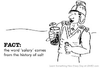
While it may appear quite clear to us now what counts for money and how it is measured, this was not always the case. Roman soldiers used to be paid in salt (in Latin: salarium, or salary), hence the saying "that a man is worth his salt." And Native Americans used wampum beads as currency. Different cultures have historically adopted different forms of money believing it to be more efficient than a pure barter system.

Money is defined by its ability to serve as a medium of exchange (just about everyone will accept US dollars, but not many will accept salt these days for payment), unit of account (with fiat money [notes & coins] we know exactly how much something is worth to the decimal point), and store of value (it would be unwise to choose a perishable item, such as ice cream, as money since it would be problematic to store). Interestingly, what counts as money is constantly evolving. Some argue for a global digital currency. In 2008 China rebuffed US economic pressure when they threatened to "diversify" their reserve currency away from US dollars and toward "Special Drawing Rights (SDR)" - a weighted-basket of 4 currencies (dollar, euro, yen, and pound) held at the IMF. China currently holds $2 trillion in US dollar reserves - more than any other country.

Now that we know what constitutes money, how governments measure the money supply, and the desired goal of economic policy, we can look deeper into the three methods the Fed uses to control the money supply. Perhaps most important, the Fed constantly buys and sells US Treasuries through the FOMC (Federal Open Market Committee). When the Fed buys Treasuries on the open market they are paying for those notes with dollars that are then circulated through the economy, thus increasing the money supply (somewhat similar to Microsoft buying back company shares on the stock market). In contrast, if the FOMC were to sell Treasuries, then they would be collecting money from investors, essentially taking money out of circulation, thus decreasing supply.

The Fed also influences money supply by regularly adjusting the discount rate, the benchmark rate that banks must pay to borrow directly from the Fed. The discount rate currently stands at 0.50%. The Fed would prefer that banks borrow from each other, and they do so through the federal funds rate, which currently charges 0.25% when banks borrow from each other for overnight lending. Also tied to the discount rate is the prime rate, currently at 3.25%, which is the rate banks typically charge to their best business customers. But they all take their lead from changes in the discount rate.

Finally, the Fed sets the reserve requirements that each bank must keep on deposit rather than lend out. The current reserve requirement may not change for years. Currently the reserve ratio stands at 10% where it has been since 2006. The reserve ratio also affects the money multiplier effect since only a bank's "excess reserves" may re-enter the economy in the form of loans. The formula for the money multiplier is:

(1 + a) / (a + b)
where "a" the "currency drain ratio" (% of consumer cash not held in banks)
where "b" the "desired reserve ratio" (set by the Fed)
Using the date from above, we have:
(1 + .50) / (0.50 + 0.10)
= 1.50 / 0.60
= 2.5 (for every $1 deposited in a bank, $2.50 can be lent out)

While most of this post deals with monetary policy, current US Treasury Secretary, Tim Geitner, might argue otherwise. Through the Treasury Department the government can influence aggregate demand and supply by adjusting tax rates and through government spending programs. The $700 billion TARP program stands alone as the largest of all government spending programs. Many economists continue to disagree whether or not monetary and fiscal policy are effective (Keynesians), or if they just aggravate conditions moreso than if left alone (monetarists).

pre-mba: oxford grading system

Lately I've been posting a lot of blogs about studying for the CFA. After all, I do mention that the goal of my blog is to guide you through "admission strategies to surviving the core curriculum to securing your dream job," and I cannot think of a better review for the MBA core curriculum then the CFA, which focuses on accounting, economics, and finance. While I will continue such posts, I thought it would be nice for a change to talk more about the Oxford MBA grading system.

Schools like Oxford are brimming with over-achievers. The average undergraduate degree earned by an applicant entering into the Oxford MBA is a "second first class degree" (also known as a 2:1, or a 3.50 GPA). The highest class degree awarded by Oxford University is the coveted "first class degree" (also known as a 1:1, or a 3.80+ GPA). For MBA students the class of degree that you graduate with is ultimately determined by your number score.

Distinction level:
80-100 Superb work
75-79 Excellent work
70-74 Fine work

Pass level:
65-69 Strong pass
55-64 Good pass
50-54 Pass

Fail:
45-49 Marginal fail
0-44 Outright fail

The World Education Services boasts a wonderful website where you can get a good approximation for converting grades from any country. For example, a student studying at an American college might earn a 88% in a class, which translates into a B+ grade, or a 3.50 GPA. The process is somewhat similiar in British universities, except there is not as much grade inflation, so a 65% might be considered a B+, which is good enough to earn you a 2:1. As students scramble for the top of their class, what exactly makes the grade & perhaps more importantly, does it even matter?

Oxford MBA students will take approximately 18 courses during the three terms they are there. In practice, the range of grades earned are from 40% to 80%. Students must score a minimum passing grade of 50%. Most strive for a 70%+ mark since this begins the various gradations of "distinction." The average mark achieved by students is a 63% "second class degree" (also known as a 2:2, or 3.33 GPA). Students who score a 70%+ grade in at least one class during any of the academic terms makes the Dean's List, and are often invited to a special dinner hosted by Colin Mayer (SBS Dean) and Stephan Chambers (MBA Director). Anyone looking to graduate with overall distinction must get a 70%+ in at least 6 of their 18 courses. Only 10% of Oxford MBA students achieve this feat. So, what is the good news?

Oxford proves the old adage that the hardest part of getting an MBA is getting into the school. It's true. Almost no one fails. In a recent MBA class, 231 out of 234 students graduated with their MBA. Out of the 3 that did not graduate, one outright failed and the remaining two left the program. While the exact reasons for the three that did not graduate are unknown, we can be reasonably confident that 99% of students who begin the course will pass. Further, past Oxford MBA students tell me that often the most interesting jobs went to those students who may have even had to "re-sit" an exam because they failed it the first time. Grades only matter for a few top employers, and also for those students wishing to land their top choice "Strategic Consulting Projects (SCP)" during the summer.


So by all means work hard, and for heaven's sake, hand in all your assignments on time and show up for your final exams! But when you feel that the stress is piling on top of you...sit back...take a deep breath...imagine the dreaming spires that surround you...and relax. Realize that in time all things will pass (including you and the MBA course), and you will get a good job.

cfa study session #4: economics: elasticity

Following quantitative methods comes an entire 500 page book devoted exclusively to economics. Separated into 3 sections, the economics portion of the CFA exam focuses on microeconomics, macroeconomics, and monetary & fiscal policy. This blog post will deal specifically with the first section: microeconomics, which includes price elasticity, market theory, and the organization of production & output.

We start with understanding the "price elasticity of demand," which simply measures the responsiveness of the quantity demanded of a product relative to changes in the price for that same product. This degree of responsiveness determines how elastic the products is, that is, whether it is elastic (very responsive), inelastic (not responsive), or unit elastic (when change in demand equals change in price). The equation is:

elasticity of demand = *% change in quantity demanded / % change in price
* % change is calculated by dividing the difference between the starting and ending values by an average of the starting and ending values (rather than dividing by the beginning value, which is more common when calculating % changes) to get a more accurate elasticity ratio.

Intuitively we know that some products, such as oil, are highly inelastic. In other words, the world will always demand oil regardless of the price, as evidenced when a barrel of oil reached an all-time peak of $147.27 on July 11, 2008. In contrast, a product such as a t-shirt is very elastic. Unless it's a Ralph Lauren polo t-shirt, most people consider one t-shirt to be very similar to any other, and therefore will purchase from whichever manufacturer has the lowest price. Elasticity isn't always a foregone conclusion, and it can change over time. For example, when Apple launched the iPod they successfully differentiated their mp3 from their competitors, turning an otherwise elastic commodity into an inelastic "must-have" brand. By developing a strong brand image and brand loyalty, Apple was able to charge a premium by changing the elasticity for their iPod.

Products tend to be elastic when there a large number of substitutes available. For example, an increase in the price of hamburgers will lead to a decrease in their consumption, because hamburgers have an elastic demand curve, and an concomitant increase in consumption of hot dogs (all other things being equal), because hot dogs are consider a viable substitute for hamburgers. There is no accounting for taste! This example sets the stage for the next step in understanding elasticity, which is calculating "cross elasticity" to determine the responsiveness of demand relative to price based on more than one product, such as hamburgers and hot dogs.

Using the above example, we can calculate whether two different products are substitutes (positive cross elasticity) or compliments (negative cross elasticity). If the price of hamburgers doubles from $2 to $4 each, and this results in an increase in hot dogs consumed from 8 to 14, then we can calculate that the two products are substitutes, because resulting cross elasticity ratio is positive .817, calculated as follows:

= (8-14)/11 / (4-2)/3
= 5.45% / 6.67%
cross elasticity = .817

The higher the number, the more magnified the difference in quantity demanded in one good relative to an incremental change in price of the substitute good. And of course the same holds true working in reverse for compliment goods, such as soda and hotdogs, which we would expect to have a negative cross elasticity.

Besides measuring the elasticity of demand, and cross elasticity, we can similarly calculate "income elasticity" by dividing the % change in quantity demanded of a product by a % change in income. In other words, when we earn more money we are more likely to purchase "luxury" products (i.e. steak and lobster), which have high elasticity, and less likeley to purchase inelastic "inferior" products (i.e. potatoes and rice). In this case a negative ratio indicates an inferior good, and a positive ratio indicates a luxury good, which is highly responsive to changes in income and therefore very elastic.

Elasticity of supply operates along similar lines as it does for demand. We calculate supply elasticity by dividing the % change in quantity supplied by the % change in price. The degree of responsiveness of supply to price often depends on the number of substitutes available, and whether the time-frame for making a supply decision is momentary, short-term, or long-term in nature.

Beyond asking you to calculate elasticity, a typical question may involve understanding the effect of elasticity on demand and revenue. For example, "For a particular company's product, the % change in quantity demanded is smaller than the % change in price that caused the change in quantity demanded. If the company increased the price of that product, total revenue from sales of that product would most likely:
A. increase and demand in elastic
B. decrease and demand is elastic
C. increase and demand is inelastic

The answer is C. We must first determine whether or not the product is elastic or inelastic before we can determine its effect on quantity demanded and ultimately revenue. The question tells us that price has little effect on quantity demanded (in fact, it's smaller!). If a product is inelastic then people will continue to buy it even if the price goes up (like the price of oil). Therefore, even if the same amount of product is sold, but the price they are charging has increased, then by definition the total revenue must also increase.